- 以 QuPath 检测 NeuN 阳性神经元,结合空间形态计量特征,量化 FCD 的皮质构筑异常。
- 测试集标本总体诊断准确率为 88.2%,亚区分类准确率为 70.6%。
- EEG 异常但组织学“看似正常”的皮质,呈现与 FCD 邻近区相似的紊乱,有别于尸检对照。
摘要
对于缺乏磁共振成像可见病灶(如局灶性皮质发育不良,FCD)的癫痫患者,外科切除以脑电图(EEG)活动异常区域为靶点。然而,在这些标本中通过组织病理学识别细微的皮质构筑异常仍有困难。我们研究了基于人工智能(AI)的 NeuN 染色皮质切片形态计量及空间分析,能否检出癫痫切除标本中的神经元构筑紊乱,包括组织学上无明确发育不良的区域。研究从 83 个 FCD 区域及 19 例神经系统正常的尸检对照生成全切片图像。在 QuPath 中将感兴趣区标注为 FCD、FCD 邻近区、FCD 远隔区、看似正常区(EEG 异常但组织学无发育不良)及真正正常区(尸检对照)。利用 QuPath 检测 NeuN 阳性神经元,敏感度为 90%,假阳性率为 12%。提取神经元聚集、分布不均一性和核形态等空间及形态计量特征,用于训练经最小绝对收缩与选择算子正则化的多项回归分类器。分类器对亚区分类的准确率为 70.6%,对标本总体诊断的准确率为 88.2%。值得注意的是,EEG 异常但组织学无发育不良的区域呈现可量化的构筑紊乱,与 FCD 邻近区域相似,而不同于对照组织。AI 驱动的神经元形态和空间分布分析揭示了癫痫切除标本中细微的皮质紊乱,包括组织学难以明确判断的区域。仍需进一步研究,以确定该方法能否提高神经病理评估的诊断检出率,并支持更精确的癫痫手术靶区定位。
引言
约三分之一的癫痫患者存在药物治疗难以控制的发作 [1],并伴随较差的社会经济及临床结局 [2]。在药物难治性局灶性癫痫患者中,局灶性皮质发育不良(FCD)和海马硬化是最常见的基础病变,两者均可能适合外科切除 [3]。虽然大多数致痫灶可由磁共振成像(MRI)检出,但部分患者的病灶在 MRI 上呈阴性。这些 MRI 阴性病例的外科切除以脑电图(EEG)异常活动灶为靶点。然而,这类病例接受切除手术的可能性较低,且术后无发作结局也较差 [4, 5, 6]。
FCD 的组织病理学分类可提供大量预后信息,组织学确诊 FCD 提示手术结局较好。国际抗癫痫联盟(ILAE)将 FCD 分为三大类:
- FCD 1 型(FCD 1):皮质构筑扭曲,不伴畸形神经元或气球细胞。
- FCD 2 型(FCD 2):
- 构筑异常伴畸形神经元(FCD 2A);
- 构筑异常伴畸形神经元和气球细胞(FCD 2B)。
- FCD 3 型:与另一主要病变相关的构筑异常 [7]。
外科切除标本以所识别的最具包容性的 FCD 类别作为总体组织病理诊断,即以观察到的最高类别作为总体诊断。关键在于,不同 FCD 亚型的手术结局不同;确诊 FCD 1 的患者约 50% 在 1 年时达到 Engel I 级结局,而 FCD 2 为 69% [8, 9]。在 MRI 阴性病例中,组织病理诊断对于确定基础病因及判断预后尤为重要。
尽管意义重大,FCD 的组织学诊断仍面临挑战。ILAE 标准在日常实践中可能难以应用,导致显著的观察者间差异及诊断不确定性 [10, 11]。此外,约 5%–10% 的局灶性癫痫外科切除病例在组织病理检查中未发现基础病变,凸显了 FCD 组织学诊断的难度 [8, 12]。虽然近年来分子诊断的进展已识别出与皮质发育畸形相关的体细胞及胚系突变,但这些发现主要有助于诊断较明显的 FCD 2 病变,对检出更细微异常的作用有限 [13]。
这些挑战凸显了采用客观、可重复工具辅助评估癫痫切除标本组织病理的必要性 [14]。为此,我们研究利用人工智能(AI)量化的细胞形态及神经元分布特征建立机器学习分类器,能否辅助发现提示 FCD 的细微构筑异常。我们将这一方法用于缺乏明确皮质发育不良 MRI 证据的癫痫切除队列,以 AI 量化皮质构筑及神经元细胞学特征,随后用于训练经最小绝对收缩与选择算子(LASSO)正则化的多项回归分类器。
材料与方法
2.1 伦理审查、标本与原始数据采集
本研究经本机构伦理审查委员会批准,并依照《赫尔辛基宣言》开展。手术切除标本来自 29 例 MRI 阴性的药物难治性局灶性癫痫患者。选取 19 例年龄匹配、神经系统健康的尸检标本,以相应皮质区域作为对照。所有组织样本均来自本机构组织档案库。一名具有专科资质的神经病理医师对所有手术病例的苏木精–伊红(H&E)染色切片进行盲法组织病理复核。按照此类病例的常规做法,依据 ILAE 2022 共识分类,以各病例所见最高程度的 FCD 进行分类。此外,由于 FCD 病变具有空间异质性,不同组织区域可分别满足不同 FCD 类别的诊断标准 [15, 16],每个感兴趣组织亚区还依据仅在该亚区内出现的形态特征独立分类。选取代表性切片(n = 83),以反映病变的总体构筑。尸检对照经组织学复核证实无病变,并同样选取代表性切片。
所有选定切片均行 NeuN 免疫组织化学(IHC)染色(克隆 A60;Zeta 公司,美国加利福尼亚州 Sierra Madre)。对 H&E 和 NeuN 染色切片均生成全切片图像(WSI)。使用 QuPath(0.4.2 版)[17],按以下类别标注感兴趣区(ROI;图 1 及补充数据 S1):
- FCD 2A 或 2B:明确具有 FCD 2A 型或 2B 型发育不良的区域;
- FCD 邻近区:毗邻 FCD 但未受其累及的皮质;
- FCD 远隔区:构筑正常、在空间上与发育不良区分离的皮质;
- 看似正常区:以 EEG 发作起始区为靶点的癫痫切除皮质,组织学无明确发育不良;
- 真正正常区:尸检对照中组织学正常的皮质。
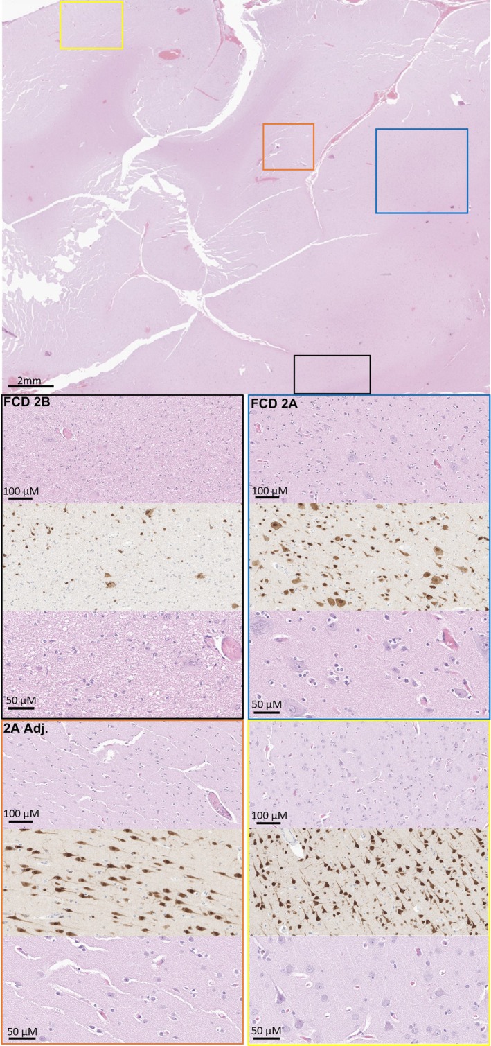
组织区域的组织学分类示意图。(上)一例 H&E 染色切片低倍图,同时展示四种不同的皮质感兴趣区,以彩色方框标示。(下)相应感兴趣区的中倍及高倍图:上排为 H&E,中排为与上排相同放大倍数的 NeuN IHC,下排为更高倍的 H&E。颜色含义如下:黑色为局灶性皮质发育不良(FCD)2B,可见气球细胞和构筑扭曲;蓝色为 FCD 2A,可见畸形神经元和构筑扭曲,但无气球细胞;橙色为紧邻明确皮质发育不良灶(本例为 FCD 2A 区域)的组织学外观正常皮质;黄色为远离病灶的组织学外观正常皮质,其间以无明显构筑及细胞学异常的区域分隔。
针对 NeuN 染色 WSI 优化 QuPath 阳性细胞检测算法,并应用于各 ROI,提取所有 NeuN 阳性神经元的位置及形态计量数据。在其中 12 个 ROI 中,以具有专科资质的神经病理医师的人工细胞分类结果验证算法性能。采用 Kruskal–Wallis 检验比较不同组织学类别间的检测性能。
2.2 特征生成、特征选择与模型构建
从 QuPath 提取所有已分类细胞的空间和形态数据,在 R(4.2.1 版)中使用 tidyverse 和 spatstat 软件包分析 [18, 19]。在各 ROI 内汇总单细胞形态计量特征,分别针对 NeuN 阳性与阴性细胞群,计算均值、中位数、最大值、最小值、标准差和极差等统计描述指标。将 NeuN 阳性细胞的空间坐标与各 ROI 对应的人工定义观察窗口结合,生成平面点模式。由此计算神经元分布的全局强度及汇总函数,包括 Ripley K 函数的线性变换 L(r)、配对相关函数 PCF(r) 和最近邻分布 G(r)(图 2 简要图解了 L(r)、G(r) 和 PCF(r) 的含义)。在所有标本中,以 513 个固定半径估计每个汇总函数,并作为模型开发的输入特征。采用高斯核(σ = 50)生成局部神经元强度的核平滑估计,其像素分辨率对应原始图像的 7 × 7 像素。由这些强度图进一步提取特征,包括全局最小值和最大值、强度热点的数量和大小(热点定义为强度超过第 99 百分位的连续像素簇)及热点轮廓(完整特征清单见补充资料 S1:数据 1)。
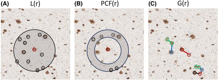
L、PCF 和最近邻 G 等二级点模式汇总函数的图形比较。(A)L 函数是 Ripley K 函数的线性变换。在感兴趣点周围生成一系列半径为 r 的圆(灰色区域),计数距该点 r 范围内的事件数。按圆面积对计数进行标准化,再以 r 为横轴绘图。对样本内多个点及多个 r 值重复该过程,从而估计样本在一系列 r 上的函数。具体而言,若该值低于完全随机点集的计算值,表示点间距大于随机预期;反之,若高于随机点集的值,则表示点较随机分布预期更为接近。(B)配对相关函数(PCF)计数一系列同心圆环(灰色区域)内的点,既不计入小于圆环最小半径的点,也不计入大于最大半径的点。排除最小圆以内的点是 PCF 与 L 函数的区别所在,可检出随半径变化的点间正向(聚集)及负向(规则化)相互作用,揭示不同半径处方向相反的点间相互作用。对于给定圆环,大于 1 的值表示该范围内点数多于随机预期,即距感兴趣点该距离处存在一定聚集;小于 1 则表示点之间相互排斥。(C)最近邻函数 G(r) 表示样本中各点至最近邻点距离的分布,图中以颜色相配的圆和线表示。绘图时表示最近邻位于距离 r 以内的细胞比例。这不同于 PCF 和 L,因为它只考虑最近距离,而非给定距离内发生的事件总数。G(r) 左移意味着在该点模式中,更高比例的点在该半径以内存在最近邻。
为减轻手术与尸检标本冷缺血时间差异的潜在混杂影响,通过计算 NeuN 阳性与阴性细胞群之间的差值及比值,对形态计量特征进行标准化。对这些衍生特征采用 Kruskal–Wallis 检验比较,随后用 Mann–Whitney U 检验进行事后两两比较。若衍生特征满足以下标准,则将其母特征排除出建模:
排除标准 A:
- 至少一个衍生特征的 Kruskal–Wallis 检验存在显著差异;
- 且尸检对照(真正正常/无癫痫发作)与手术标本之间的所有两两比较均有显著差异;
- 且各手术切除标本组之间未观察到其他有显著差异的两两比较。
或满足以下标准:
排除标准 B:
- 至少一个衍生特征的 Kruskal–Wallis 检验存在显著差异;
- 且尸检对照与各切除标本类别之间的 7 项两两比较中,至少 5 项有显著差异;
- 且衍生特征的显著两两比较中,至少一项为看似正常标本与真正正常/无癫痫发作标本之间的比较;
- 且各手术切除标本组之间未观察到其他有显著差异的两两比较。
此外,排除所有来源于 NeuN 阴性细胞形态计量的特征,以及涉及阴性细胞特征的比值或差值。这是因为阴性细胞检测算法尚未依据神经病理医师标注进行优化和验证(补充资料 S2:数据 2)。空间特征不受这一筛选过程限制,因为它们独立于染色质量和细胞保存状况。
使用 caret 软件包的 createDataPartition 函数,将病例及对照随机划分为训练集(80%)和测试集(20%),确保各组织学类别具有代表性分布。对于含多个空间分离 ROI 的病例,并未要求其所有 ROI 全部归入测试集或训练集(补充数据 S3)。采用 glmnet 软件包,以提取的特征训练 LASSO 正则化多项 logistic 回归模型。通过五折交叉验证优化正则化参数 λ,使多项分类误差最小。最终模型采用训练时误分类率最低的 λ 值所对应的特征系数,应用于预留测试集。分别依据标本总体诊断及每个 ROI 精确组织学分类的误分类率评估模型性能。
2.3 不同组织学类别间模型特征的分析与比较
对 QuPath 衍生的神经元形态特征,以及全部入选模型的不均一性相关特征,进行 Kruskal–Wallis 检验。事后两两比较采用 Mann–Whitney U 检验,并使用 Benjamini–Hochberg(BH)校正控制多重比较。
对于源于二级点模式函数 PCF(r)、L(r) 和 G(r) 的特征,采用特定半径的单个估计值作为模型特征。为更全面评估空间关系,通过置换检验比较各组在全部半径上的完整函数分布。比较包括:
- 真正正常与看似正常标本;
- 真正正常与各发育不良相关亚区(FCD、FCD 邻近区、FCD 远隔区);
- 全部发育不良相关亚区之间的相互比较。
首先对每个函数进行组间整体评估,再在适用时进行预先计划的两两比较。
结果
3.1 细胞分类器的验证与性能
在 12 个代表性组织区域,以具有专科资质的神经病理医师的人工标注为参照,评估优化后 QuPath 分类器检测 NeuN 阳性和阴性细胞的性能。采用 15 μm 的最近邻(NN)阈值,界定算法与人工参照中相互一致的细胞标注。目视检查显示,算法与人工识别的 NeuN 阳性神经元高度一致(补充数据 S4)。定量比较(表 1)显示,最近邻距离中位数的偏差很小,可能源于人工放置质心时的轻微不一致。以人工标注为参考标准,算法敏感度范围为 72.5%–96.8%,所有区域的假阳性率均低于 20%。重要的是,分类器性能在各组织学亚型间无显著差异。各标本组的敏感度与假阳性率一致(分别为 p = 0.68 和 p = 0.59;图 3),表明算法在不同皮质构筑中均表现稳健。总体而言,这些发现支持该分类器具有准确性、可推广性,且不存在系统性偏倚。
| 组织学类别 | 交叉最近邻距离中位数 | 敏感度 | 假阳性率 | F1 分数 |
|---|---|---|---|---|
| 2B 邻近区 | 1.723 | 0.725 | 0.015 | 0.835 |
| 2A 邻近区 | 2.442 | 0.936 | 0.170 | 0.880 |
| 2A 发育不良区 | 2.059 | 0.940 | 0.138 | 0.899 |
| 真正正常区 | 1.982 | 0.921 | 0.186 | 0.864 |
| 真正正常区 | 1.868 | 0.953 | 0.141 | 0.904 |
| 真正正常区 | 2.144 | 0.968 | 0.124 | 0.920 |
| 真正正常区 | 2.135 | 0.828 | 0.084 | 0.870 |
| 2A 发育不良区 | 1.716 | 0.932 | 0.193 | 0.865 |
| 2A 发育不良区 | 1.673 | 0.939 | 0.067 | 0.936 |
| 2B 发育不良区 | 2.688 | 0.820 | 0.041 | 0.884 |
| 看似正常区 | 2.337 | 0.899 | 0.155 | 0.871 |
| 看似正常区 | 1.583 | 0.941 | 0.190 | 0.871 |
| 总体 | 2.069 | 0.898 | 0.125 | 0.886 |
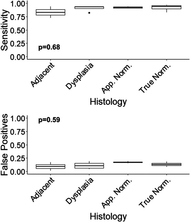
不同大类组织学类别间细胞检测算法性能的比较。(上)以神经病理专家人工标注为参照,QuPath 细胞检测算法识别 NeuN 阳性细胞的敏感度;检验统计量由 Kruskal–Wallis 检验产生,n = 12。(下)相对于神经病理专家人工标注,QuPath 细胞检测算法的假阳性率;检验统计量由 Kruskal–Wallis 检验产生,n = 12。
3.2 特征选择与模型构建
从 QuPath 提取的形态数据中,最初获得 27 个细胞层面特征,经统计汇总后,在 NeuN 阳性和阴性细胞群中形成 508 个原始及衍生的样本层面特征。排除可能受冷缺血时间差异影响的特征及源自 NeuN 阴性细胞的特征后,保留 84 个形态特征用于建模(图 S2,补充资料 S2:数据 2)。此外,每个二级点模式汇总函数生成 513 个特征,代表离散半径处的函数估计值。另生成 35 个特征,用于量化皮质神经元空间分布的不均一性。初始建模数据集共纳入 1662 个特征。
以数据集的 80% 训练 LASSO 正则化多项回归模型,通过五折交叉验证优化正则化参数 λ,使误分类误差最小(补充数据 S5)。采用最佳 λ 对应的惩罚回归系数,在剩余 20% 的测试集上评估模型性能。最终模型的性能指标汇总于表 2。分类器的总体诊断准确率为 88.2%,亚区层面的分类准确率为 70.6%。多数亚区误分类被赋予比真实标签更偏向发育不良的类别。这些发现提示,分类器可能对常规组织学不易察觉的细微构筑破坏敏感,有望在诊断不明确的病例中成为神经病理评估的补充工具。
| 亚区类别(参考标准) | 算法分类 | 诊断一致性 | 亚区一致性 | ||
|---|---|---|---|---|---|
| 真正正常区 | 真正正常区 | 是 | 是 | ||
| 真正正常区 | 真正正常区 | 是 | 是 | ||
| 真正正常区 | 真正正常区 | 是 | 是 | ||
| 看似正常区 | 看似正常区 | 是 | 是 | ||
| 2A 发育不良区 | 2A 发育不良区 | 是 | 是 | ||
| 看似正常区 | 看似正常区 | 是 | 是 | ||
| 2A 发育不良区 | 2A 发育不良区 | 是 | 是 | ||
| 2A 发育不良区 | 2A 发育不良区 | 是 | 是 | ||
| 2A 邻近区 | 看似正常区 | 否 | 假阴性 | 否 | 假阴性 |
| 2B 发育不良区 | 2B 发育不良区 | 是 | 是 | ||
| 2B 邻近区 | 2B 发育不良区 | 是 | 否 | 假阳性 | |
| 2B 发育不良区 | 2B 发育不良区 | 是 | 是 | ||
| 2A 发育不良区 | 2A 发育不良区 | 是 | 是 | ||
| 2B 远隔区 | 2B 发育不良远隔区 | 是 | 是 | ||
| 看似正常区 | 2A 发育不良远隔区 | 否 | 假阳性 | 否 | 假阳性 |
| 2A 远隔区 | 2A 发育不良区 | 是 | 否 | 假阳性 | |
| 看似正常区 | 真正正常区 | 是 | 否 | 假阴性 | |
| 准确率 | 0.882 | 0.706 | |||
3.3 模型特征分析
为更好理解分类器采用的判别特征,我们研究了形态特征在各组织学亚区间的变化。所有非零模型系数列于补充资料 S3:数据 3;各形态特征经中心化及缩放后的中位数热图见图 4,详细统计汇总见补充资料 S4:数据 4。正如预期,FCD 2B 区域具有独特的细胞形态特征谱,包括平均最小苏木精光密度(O.D.)升高、二氨基联苯胺(DAB)标准差的最大值升高、核面积中位数增大、核最大卡尺径增大及核周长增加。
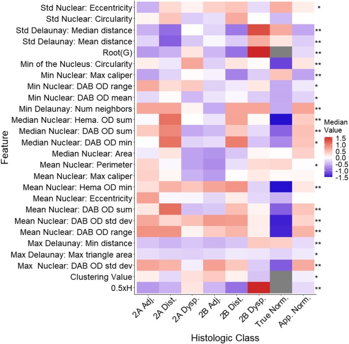
不同组织学亚区中,QuPath 衍生判别特征值中位数的热图。注意局灶性皮质发育不良(FCD)2B 和真正正常标本在形态上似与其他组织亚区不同。此外,FCD 2B 邻近区和 FCD 2A 区域在建模特征中具有相似的特征谱。看似正常区的细胞在细胞形态计量方面,与 2A 发育不良的邻近区、远隔区及 2B 发育不良远隔区显著相似,尤其体现在 DAB 和苏木精染色特征上。星号表示 Kruskal–Wallis 检验确定的显著性水平;*p < 0.05,**p < 0.001(包括两两比较在内的所有统计检验汇总见补充资料 S3:数据 3)。
有趣的是,FCD 2B 邻近区的细胞形态计量特征谱与 FCD 2A 高度相似,提示形态改变可能超出组织学界定的病变范围。同样,“看似正常”区域虽无明确组织学发育不良、但因 EEG 异常而被切除,其形态与 FCD 2A 邻近区及远隔区相似,尤其是核染色特征(图 4,补充资料 S4:数据 4)。相反,真正正常的尸检皮质在形态上似与所有手术标本不同。这些发现提示,细胞形态计量特征可能捕捉到与发育不良灶距离相关的细微空间梯度变化。
随后,我们使用非均一 L 函数、配对相关函数(PCF)和最近邻函数(G),评估 NeuN 阳性神经元之间的空间关系。对各组织学亚区绘制这些函数随半径变化的曲线,并用置换检验比较。L 和 PCF 函数在半径约 30 μm 以内均明显偏离完全空间随机性(CSR),说明成人皮质神经元分布本质上并非随机(图 5A、B)。L(r) 显示半径 <10 μm 时神经元明显离散,而 PCF(r) 提示在 15–25 μm 间存在聚集。最后,G(r) 在小半径处也显示类似离散现象,在更大距离时趋近 CSR 预期(图 5C)。
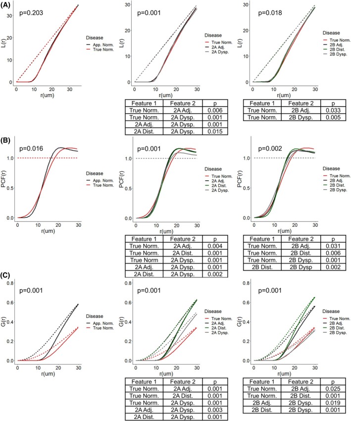
不同组织学亚区的二级点模式特征比较。(A)Ripley K 的线性变换(L)、(B)配对相关函数及(C)最近邻分布(G),均为各组织学亚区合并点模式上估计的随半径变化的函数。左列比较真正正常与看似正常区;中列比较局灶性皮质发育不良(FCD)2A 的发育不良灶、邻近区及远隔正常区;右列比较 FCD 2B 的发育不良灶、邻近区及远隔正常区。图内报告的 p 值为上述组中全部组织学亚区间的比较。虚线表示非均一空间随机点模式的汇总函数估计值。图下表格列出区域间有显著差异的两两比较。所有 p 值均以所列汇总函数的完整分布进行置换检验计算。
各组织学亚区空间汇总函数的比较分析揭示了神经元组织方式的明显差异。具体而言,与真正正常(无癫痫发作)的皮质相比,FCD 2A 及其邻近区在小半径处神经元间距更加规则,在中等距离处更突然地转为聚集(图 5A)。这一空间模式也出现在“看似正常”区,以及 FCD 2B 邻近和远隔皮质中,并反映于配对相关及最近邻分布函数(图 5B、C)。
相反,FCD 2B 区域表现出相反的空间模式:相较真正正常皮质,小半径处神经元规则化程度较低,并在更大半径时转为聚集(图 5B,右)。值得注意的是,与真正正常组织及发育不良灶邻近或远隔区域相比,FCD 2A 和 FCD 2B 的神经元聚集总体幅度均降低(图 5A、B)。这些发现提示,发育不良区虽然存在构筑紊乱,也伴有局部聚集的相对丧失,可能反映发育或退行性过程的改变。
G 函数进一步凸显两种主要模式。首先,FCD 2A 与 FCD 2B 邻近区具有相似的最近邻距离分布。其次,FCD 2B 的最近邻特征谱与真正正常皮质高度相似。这些发现提示发育不良皮质中存在复杂的空间重组:(1)发育不良区聚集减少,可能源于神经元丧失或离散;(2)邻近区聚集增加,可能反映代偿性或过渡性构筑。关键是,“看似正常”区域虽然无明显组织学异常,却呈现与发育不良邻近组织相似的空间紊乱。
鉴于各级 FCD 均由细胞学异型性与皮质构筑破坏共同定义,而这些特征本身会导致神经元分布不均一,我们生成了一组特征,以量化各 ROI 内的空间不均一性。其中,模型选出四个特征,作为组织学亚区分类的判别特征(图 6,补充资料 S1 和 S5:数据 1 和 5)。
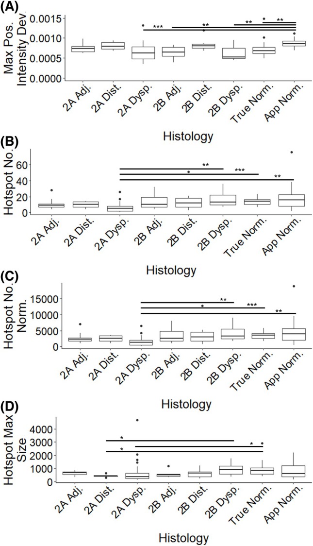
展示模型不均一性特征分布的箱线图。(A)强度最大正偏差,定义为单个最高局部核平滑强度减去全局强度。(B)热点数量,即各标本中核平滑强度达到或超过第 99 百分位的、空间上相互分离的区域数。(C)按感兴趣区总面积标准化后的热点数量。(D)热点最大面积,定义为单个感兴趣区内热点面积的全局最大值。星号表示经 Benjamini–Hochberg 方法校正的 Mann–Whitney U 检验比较的显著性:*p < 0.05,**p < 0.001,***p < 0.0001。
这些特征的分析显示,与看似正常和真正正常(无癫痫发作)皮质相比,FCD 2A 区域的不均一性显著降低。具体而言,FCD 2A 的强度最大正偏差较低、热点总数及单位面积热点数较少、平均热点面积较小(图 6)。这些发现提示,FCD 2A 的特征是神经元密度升高的区域相对较少、大小中等,且其强度偏离全局基线的程度较小,说明皮质构筑异常地更加均一。换言之,FCD 2A 似乎表现为正常成人皮质通常具有的空间不均一性程度降低。反之,看似正常区域呈现不均一性增加趋势,尤以强度最大正偏差为著(图 6A)。这提示存在局灶性神经元密度升高区域,其变化超过真正正常皮质所见的变异程度,可能反映常规组织学评估未能识别的细微构筑异常。
讨论
FCD 的诊断依赖于识别细胞学异常和皮质神经元构筑破坏,这些特征常难以检出,尤其是在 MRI 阴性癫痫病例中。AI 为整张组织切片的细胞形态及空间特征量化提供了有力手段,其精度和规模超越传统组织学评估。空间统计分析则能够发现只有同时考虑数千个细胞相对位置时才显现的神经元分布模式。在这一背景下,本研究 AI 分类器采用的特征,在概念上与神经病理医师使用的皮质构筑、核大小和形状等特征一致,但精度和范围不同。例如,平均核周长可直接对应常规组织学中的视觉评估,而配对相关函数或空间不均一性指标等,则是常规显微镜观察无法获得的、通过数学计算得出的神经元组织方式描述量。我们假设,整合这些 AI 衍生细胞学与空间特征的分类器能够发现与 FCD 相关、细微但具有诊断意义的模式。
本研究 LASSO 正则化多项回归模型确实达到了 88.2% 的总体诊断准确率及 70.6% 的亚区分类准确率。这些结果与 Kubach 等的报道相当:该研究使用卷积神经网络区分 FCD 2B 与结节性硬化症复合征中的皮质畸形,在二分类任务中达到 91% 的准确率 [20]。值得注意的是,我们的模型虽然使用了更简单的统计框架,且处理更复杂的多类别分类问题,仍获得相近性能。
重要的是,分类器能够区分真正正常(无癫痫发作)的皮质与药物难治性癫痫患者中无明确组织学异常的组织。此外,模型倾向于将不明确的亚区归为与发育不良灶更接近的类别,提示其可能对低于常规组织病理检出阈值的细微构筑变化敏感。这些发现可能与以下假说有关:发育不良相关改变超出组织学界定的病变边界,并可能参与邻近或看似正常皮质的致痫性。
最引人关注的观察或许是:癫痫患者“看似正常”皮质的空间特征与发育不良邻近区高度相似。关键在于,神经系统健康尸检对照标本的皮质区域未见这些改变。鉴于本研究细胞检测算法在手术与尸检标本中性能一致,这些发现由组织处理伪影造成的可能性较低。它们可能反映未经辅助的常规组织学检查未能捕捉到的细微皮质异常。另一种可能是,它们代表慢性癫痫活动诱导的继发改变。无论哪种情况,均需进一步研究以确定这些特征的可靠性及意义。
若得到充分验证,这些发现将具有重要的临床及生物学意义。从诊断角度看,空间分析衍生特征可为组织学表现细微的病例提供 FCD 病变的客观证据,提高诊断的可重复性和信心,并增加癫痫切除标本的诊断检出率,尤其适用于 MRI 阴性病例。除更可靠的疾病分类有助于预后判断外,可靠识别符合 FCD 的细微空间改变,还可促进深入研究残余发育不良区域的预后意义,与当前致痫区可能超出核心病灶的假说相呼应。最后,这些特征可能提高定位并分离发育不良灶的能力,从而更简便、更确切地完成细微 FCD 病变的分子特征分析;后者仍是理解 FCD 1 型病因的重要障碍。
然而,本研究目前的发现属于初步结果,其意义因此仍带有一定推测性。需要在大型癫痫切除队列中验证,纳入具有多样病变的患者、尸检对照,以及在可能情况下因其他疾病接受手术切除的非癫痫脑组织,以确定本研究观察结果对 FCD 的特异性和敏感性程度。相应地,此类研究也可能识别出与慢性癫痫活动相关、而非与某一特定基础病因相关的变化。若结果得到验证,还必须通过空间参数与患者术后结局的详细关联分析,探索这些观察的临床意义。
本研究发现也凸显了空间分析作为理解癫痫皮质组织方式工具的潜力。虽然 FCD 中神经元的空间分布尚未得到广泛研究,但既往工作已显示 FCD 2 病变中胶质细胞及血管空间模式的改变 [21, 22, 23]。例如,研究发现,与病灶周围组织相比,发育不良皮质的少突胶质前体细胞密度降低、微血管密度升高 [24]。这些观察结合本研究结果,提示神经元、胶质细胞与血管之间的空间关系可为诊断和机制认识提供丰富信息。
虽然本研究分类器在相对较小的训练集和测试集中表现良好,但仍有若干途径可改善模型性能与可推广性。当前方法将神经元点模式建模为平稳、非均一、各向同性的点过程。这一做法假定各向同性,即空间关系在各方向上均匀。未来模型可纳入各向异性空间特征,以捕捉神经元相互作用可能存在的方向性 [25]。同样,本研究分类器将二级点模式汇总函数(如 L(r)、PCF(r))的离散估计值作为特征。在后续分析中,我们观察到这些函数的变化率在不同组织学亚区间不同,提示其导数可能提供进一步的判别能力。将此类动态空间指标纳入扩展的特征空间,可能提高模型对细微构筑差异的敏感性。
在建模方面,我们选择 LASSO 正则化多项回归,是因为它具有可解释性,并适用于样本量有限的高维数据。然而,更复杂的分类器,如随机森林、梯度提升树或卷积神经网络,可能取得更佳性能,尤其是在更大的数据集中。随着对这一特征空间理解的深入,可探索这些方法以开发更稳健的模型。
另一项局限是 ROI 的人工标注,既耗时,又可能引入变异并稀释发育不良相关特征。通过算法分割或弱监督学习实现 ROI 自动选择,可能提高临床应用的可重复性及可扩展性。
采用尸检组织作为“真正正常”对照也值得考虑。虽然所选尸检标本确保无神经病理病变,并与手术病例取样的皮质区域匹配,但组织处理及死后间隔的差异可能影响细胞形态计量特征。尽管我们尝试排除对冷缺血时间敏感的特征以减轻影响,进一步验证(可能采用动物模型)仍有助于澄清死后改变对模型的影响。同样,在尸检对照之外加入其他对照材料,如因非癫痫原因切除的无病变组织,可能有助于识别各类材料中存在的重要混杂因素。
值得注意的是,本数据集未明确纳入 FCD I 型,原因是在常规手术标本中难以有把握地诊断这些区域。为此,我们纳入“看似正常”及“发育不良邻近”区域,以覆盖可能低于 FCD 明确诊断阈值的一系列皮质异常。可能需要规模更大、经共识分类并结合无监督聚类的队列,才能界定 FCD 1、微发育异常及相关病变的特异性特征。最后,本研究关注的病变范围相对较窄。未来工作应将分类器扩展至其他癫痫相关病变,如海马硬化、内侧颞叶硬化、FCD III 型及结节性硬化症复合征。这将扩大其诊断适用范围,并进一步检验特征集的可推广性。
综上,我们建立了基于 AI 量化神经元细胞形态计量及空间分布特征的 FCD 组织形态分类器。模型在训练集及测试集中显示出有前景的性能,提示该方法具有临床应用潜力。此外,对最具判别力特征的分析揭示了不同组织学亚区间的变化趋势,经进一步研究可能证实其与 FCD 的基础生物学有关。随着在更大、更多样的队列中持续完善和验证,这一方法最终可能提高癫痫外科神经病理评估的诊断精度及预后价值。
Abstract
In epilepsy patients lacking magnetic resonance imaging‐visible lesions such as focal cortical dysplasia (FCD), surgical resections target regions with abnormal electroencephalographic (EEG) activity. However, histopathological identification of subtle cortical architectural abnormalities in these specimens remains challenging. We investigated whether artificial intelligence (AI)‐based morphometric and spatial analysis of NeuN‐stained cortical sections could detect neuronal architectural disorganization in epilepsy resections, including regions without definitive histologic dysplasia. Whole slide images were generated from 83 FCD regions and 19 neurologically normal autopsy controls. Regions of interest were annotated in QuPath as FCD, FCD‐adjacent, FCD‐distant, apparently normal (abnormal EEG without histologic dysplasia), and true normal (autopsy controls). NeuN‐positive neurons were detected using QuPath (90% sensitivity, 12% false positive rate). Spatial and morphometric features—including neuronal clustering, distribution inhomogeneity, and nuclear morphology—were extracted and used to train a multinomial, Least Absolute Shrinkage and Selection Operator‐regularized regression classifier. The classifier achieved 70.6% accuracy in subregion classification and 88.2% accuracy in overall specimen diagnosis. Notably, regions with abnormal EEG but lacking histologic dysplasia exhibited quantifiable architectural disorganization similar to those seen in areas adjacent to FCD and distinct from control tissue. AI‐driven analysis of neuronal morphology and spatial distribution reveals subtle cortical disorganization in epilepsy resections, including in histologically ambiguous regions. Further investigation is warranted to determine if this methodology can enhance the diagnostic yield of neuropathological evaluation and support more precise surgical targeting in epilepsy.
INTRODUCTION
Approximately one third of patients with epilepsy have seizures that are resistant to medical management [1] which is associated with poor socioeconomic and clinical outcomes [2]. Among patients with drug‐resistant focal epilepsy, focal cortical dysplasia (FCD) and hippocampal sclerosis are the most common underlying pathologies, both of which may be amenable to surgical resection [3]. While the majority of epileptogenic foci are detected by magnetic resonance imaging (MRI) studies, a subset of patients has MRI‐negative foci. In these MRI‐negative cases, surgical resections target foci of abnormal electroencephalographic (EEG) activity. However, surgical resection in these cases is less likely to be performed, and post‐surgical outcomes are less favorable in terms of seizure freedom [4, 5, 6].
The histopathologic classification of FCD yields considerable prognostic information, and the histologic diagnosis of FCD portends favorable surgical outcomes. The International League Against Epilepsy (ILAE) classification defines three overarching classes of FCD:
FCD type 1 (FCD 1): Cortical architectural distortion without dysmorphic neurons or balloon cells,
FCD type 2 (FCD 2):
architectural abnormalities with dysmorphic neurons (FCD 2A)
Architectural abnormalities with dysmorphic neurons and balloon cells (FCD 2B), and
FCD type 3: (architectural abnormalities associated with another principal lesion) [7].
The surgically resected samples are assigned to the most inclusive class of FCD identified as the overall histopathologic diagnosis (i.e., the overall diagnosis is that of the highest class of FCD observed). Critically, surgical outcomes vary by FCD subtype; approximately 50% of patients diagnosed with FCD 1 achieve Engle class I outcomes at 1 year compared to 69% for FCD 2 [8, 9]. In MRI‐negative cases, histopathological diagnosis becomes especially critical for identifying the underlying etiology and informing prognosis.
Despite its importance, the histological diagnosis of FCD remains challenging. The ILAE criteria can be difficult to apply in routine practice, leading to substantial interobserver variability and diagnostic uncertainty [10, 11]. Moreover, histopathologic examination fails to reveal an underlying lesion in approximately 5%–10% of surgically resected focal epilepsy cases, highlighting the challenge of histologic diagnosis of FCD [8, 12]. While recent advances in molecular diagnostics have identified somatic and germline mutations associated with malformations of cortical development, these findings have primarily aided in the diagnosis of more overt FCD 2 lesions, with limited utility in detecting subtler abnormalities [13].
These challenges underscore the need for objective, reproducible tools to support the histopathological evaluation of epilepsy resections [14]. To this end, we investigated whether a machine learning classifier utilizing artificial intelligence (AI)‐quantified features of cytomorphology and neuronal distribution could assist in detecting subtle architectural abnormalities suggestive of FCD. We applied this approach to a cohort of epilepsy resections lacking definitive MRI evidence of cortical dysplasia, using AI to quantify cortical architectural and neuronal cytological features which were subsequently used to train a Least Absolute Shrinkage and Selection Operator (LASSO)‐regularized multinomial regression classifier.
MATERIALS AND METHODS
Institutional Review Board, specimens, and raw data collection
This study was approved by our Institutional Review Board and conducted in accordance with the Declaration of Helsinki. Surgical resection specimens were obtained from 29 patients with MRI‐negative, drug‐resistant focal epilepsy. Nineteen age‐matched, neurologically healthy autopsy specimens from comparable cortical regions were selected as controls. All tissue samples were obtained from our tissue archives. A blinded histopathological review of hematoxylin‐and‐eosin (H&E) stained sections from all surgical cases was performed by a board‐certified neuropathologist. Each case was classified according to the ILAE 2022 consensus classification for the most advanced degree of FCD present, as routinely performed for these cases. Additionally, because FCD lesions are spatially heterogenous with distinct tissue regions fulfilling diagnostic criteria for different classes of FCD [15, 16] each tissue subregion of interest was independently classified according to the morphologic features present only within that subregion. Representative sections (n = 83) were selected to reflect the overall lesional architecture. Autopsy control cases were confirmed to be non‐lesional by histological review, and representative sections were similarly selected.
All selected sections underwent immunohistochemical (IHC) staining for NeuN (clone A60; Zeta Corp., Sierra Madre, CA). Whole‐slide images (WSIs) of both H&E and NeuN‐stained sections were generated. Using QuPath (version 0.4.2) [17], region of interest (ROIs) were annotated as follows: (Figures 1 and Data S1):
FCD 2A or 2B—regions with definitive FCD type 2A or FCD type 2B dysplasia,
FCD‐adjacent—cortex adjacent to but not involved by FCD,
FCD‐distant—cortex with normal architecture, spatially separated from dysplasia,
Apparently normal—cortex from epilepsy resections targeting EEG ictal onset zones, without definitive histologic dysplasia, and
True normal—histologically normal cortex from autopsy controls.
Schematic of histologic classification of tissue regions. (Top) Low‐power image of an H&E‐stained section from a case exemplifying all four distinct cortical regions of interest, highlighted by colored boxes. (Bottom) Intermediate and high‐power views of corresponding regions of interest, showing H&E (top), NeuN IHC (middle) at same magnification as top and higher‐power (H&E bottom). Color coding is as follows: black focal cortical dysplasia (FCD) 2B, demonstrating balloon cells and architectural distortion; blue FCD 2A, demonstrating dysmorphic neurons and architectural distortion, but lacking balloon cells. Orange Histologically normal‐appearing cortex immediately adjacent to foci demonstrating obvious cortical dysplasia (regions of FCD 2A, in this case). Yellow: Histologically normal‐appearing cortex distant from lesional foci and separated by areas lacking obvious architectural and cytologic abnormality.
The QuPath positive cell detection algorithm was optimized for NeuN‐stained WSIs and applied to each ROI to extract positional and morphometric data for all NeuN‐positive neurons. Algorithm performance was validated against manual cell classifications performed by a board‐certified neuropathologist on a subset of 12 ROIs. Detection performance across histologic categories was compared using Kruskal–Wallis tests.
Feature generation, feature selection, and model generation
Spatial and morphologic data for all classified cells were extracted from QuPath and analyzed in R (version 4.2.1) using tidyverse and spatstat packages [18, 19]. Morphometric features of individual cells were aggregated within each ROI and summarized using statistical descriptors including mean, median, maximum, minimum, standard deviation, and range, across both NeuN‐positive and ‐negative cell populations. Spatial coordinates of NeuN‐positive cells, along with manually defined observation windows corresponding to each ROI, were used to generate planar point patterns. These patterns were used to calculate the global intensity of the neuronal distribution, and summary functions including L(r), a linear transformation of Ripley's K function, Pair correlation function, PCF(r), and the nearest‐neighbor distribution, G(r) (Figure 2 provides a brief graphical guide to the interpretation of L(r), G(r), and PCF(r)). Each summary function was estimated at 513 fixed radii across all specimens and used as input features for model development. Kernel‐smoothed estimates of local neuronal intensity were generated using a Gaussian kernel (σ = 50) with pixel resolution corresponding to 7 × 7 pixels of the original image. From these intensity maps, additional features were extracted, including global minima and maxima, number and size of intensity hotspots (defined as contiguous pixel clusters exceeding the 99th percentile of intensity), and hotspot contours (see Supporting Information S1: Data 1 for a complete feature list).
Graphical comparison of the L, PCF, and G nearest‐neighbor secondary point pattern summary functions. (A) The L function is a linear transformation of the Ripley's K function. Here a series of circles of radius “r” (gray area) surrounding a point of interest are generated and the number of events falling within “r” distance of the point of interest are counted. The number is normalized to the area of the circle and plotted against the value of “r.” The procedure is repeated for many points within the sample and many values of “r” to generate an estimate of the function for the sample across a range of “r.” More concretely, if this value is below the value calculated for a completely random set of points it means that the points are spread farther apart than would be expected at random; conversely if it is higher than the value calculated for a random set of points it means that points are occurring more closely together than would be expected under random distribution. (B) The pair correlation function (PCF) counts the points falling within a series of concentric rings (gray area) such that points falling within the smallest radius of the ring and outside the largest radius are not included in the count. The exclusion of points within the smallest ring accounts for the difference between PCF and L functions and allows for the detection of positive (clustering) and negative (regularization) interactions of points that differs according to radii such that interpoint interactions of opposite directions at different radii are unmasked. Here, a value greater than one for any given ring signifies increased points falling in that range over what is expected randomly (a degree of clustering at that distance from the point of interest) while a value below one represents repulsion of points from each other. (C) The nearest‐neighbor function (G(r)) represents the distribution of the distances of a sample of points to their nearest‐neighboring point, denoted in the image by color‐matched circles and lines. The function is plotted as the proportion of cells with a nearest neighbor lying within a distance “r.” This is distinct from both PCF and L as only the closest distances are considered rather than the total number of events occurring within a given distance. A left shift G(r) indicates a higher proportion of points in the shifted pattern that have a nearest neighbor present within that radius.
To mitigate potential confounding effects of differential cold ischemic time between surgical and autopsy specimens, morphometric features were normalized by calculating the difference and ratio between NeuN‐positive and ‐negative cell populations. These derivative features were statistically compared using Kruskal–Wallis tests, followed by post hoc pairwise comparisons using Mann–Whitney U tests. Parent features were excluded from modeling if their derivative features met the following criteria:
Exclusion Criteria A
Significantly different Kruskal–Wallis test for at least one derivative feature,
AND
All pairwise comparisons between autopsy controls (true normal/non‐seizure) and surgical specimens were found to be significant,
AND
No additional significant pairwise comparisons were observed between surgically resected specimen groups.
OR
Exclusion criteria B
Significantly different Kruskal–Wallis test for at least one derivative feature,
AND
At least five of seven significant pairwise comparisons between autopsy controls and resected specimen categories,
AND
At least one significant pairwise comparison of derivative features being the comparison between apparently normal and true normal/non‐seizure specimens,
AND
No additional significant pairwise comparisons were observed between surgically resected specimen groups.
Additionally, all features derived from NeuN‐negative cell morphometry, or from ratios or differences involving negative‐cell features, were excluded. This was because of the lack of optimization and validation of the negative‐cell detection algorithm against neuropathologist annotations (Supporting Information S2: Data 2). Spatial features were exempt from this filtering process, as they are independent of staining quality and cell preservation.
Cases and controls were randomly partitioned into training (80%) and test (20%) sets using the createDataPartition function from the caret package, ensuring representative distribution across histologic categories. Cases with multiple, spatially distinct regions of interest were not restricted to fall entirely within the test or training sets (Data S3). A LASSO‐regularized multinomial logistic regression model was trained on the extracted features using the glmnet package. The regularization parameter (λ) was optimized via five‐fold cross‐validation to minimize multinomial classification error. The final model was applied to the held‐out test set using the feature coefficients corresponding to the λ value that minimized misclassification in training. Model performance was assessed based on misclassification rates for both overall specimen diagnosis and exact histologic classification within each ROI.
Analysis and comparison of model features across histologic classifications
Neuronal morphologic features derived from QuPath, along with all inhomogeneity‐related features selected for model inclusion, were statistically analyzed using Kruskal–Wallis tests. Post hoc pairwise comparisons were performed using Mann–Whitney U tests, with Benjamini–Hochberg (BH) correction applied to control for multiple comparisons.
For features derived from secondary point pattern functions—PCF(r), L(r), and G(r)—individual estimates at specific radii were used as model features. To assess spatial relationships more comprehensively, the full distributions of these functions across all radii were compared between groups using permutation tests. Comparisons were conducted between the following regions:
True normal and apparently normal specimens;
True normal and each dysplasia‐associated subregion (FCD, FCD‐adjacent, FCD‐distant); and
All dysplasia‐associated subregions against one another.
Each function was first evaluated in a group‐wise manner, followed by planned pairwise comparisons where applicable.
RESULTS
Validation and performance of the cell classifier
The performance of the optimized QuPath classifier for NeuN‐positive and ‐negative cell detection was evaluated against manual annotations performed by a board‐certified neuropathologist on 12 representative tissue regions. A nearest‐neighbor (NN) threshold of 15 μm was used to define concordant cell annotations between the algorithm and manual reference. Visual inspection demonstrated a high degree of concordance between algorithmically and manually identified NeuN‐positive neurons (Data S4). Quantitative comparison (Table 1) revealed minimal deviations in median nearest‐neighbor distances, likely attributable to minor inconsistencies in manual centroid placement. Sensitivity of the algorithm ranged from 72.5% to 96.8%, with false positive rates consistently below 20% across all regions, using manual annotation as the reference standard. Importantly, classifier performance did not significantly differ across histologic subtypes. Sensitivity and false positive rates were consistent among all specimen groups (p = 0.68 and p = 0.59, respectively; Figure 3), indicating that the algorithm performs robustly across a spectrum of cortical architectures. Collectively, these findings support that the classifier is accurate, generalizable, and lacks systematic bias.
| Histology | Median Cross NN Dist. | Sensitivity | False positive rate | F1‐score |
|---|---|---|---|---|
| 2B_adjacent | 1.723 | 0.725 | 0.015 | 0.835 |
| 2A_adjacent | 2.442 | 0.936 | 0.170 | 0.880 |
| 2A_dysplasia | 2.059 | 0.940 | 0.138 | 0.899 |
| True normal | 1.982 | 0.921 | 0.186 | 0.864 |
| True normal | 1.868 | 0.953 | 0.141 | 0.904 |
| True normal | 2.144 | 0.968 | 0.124 | 0.920 |
| True normal | 2.135 | 0.828 | 0.084 | 0.870 |
| 2A_dysplasia | 1.716 | 0.932 | 0.193 | 0.865 |
| 2A_dysplasia | 1.673 | 0.939 | 0.067 | 0.936 |
| 2B_dysplasia | 2.688 | 0.820 | 0.041 | 0.884 |
| Apparent normal | 2.337 | 0.899 | 0.155 | 0.871 |
| Apparent normal | 1.583 | 0.941 | 0.190 | 0.871 |
| Overall | 2.069 | 0.898 | 0.125 | 0.886 |
Comparison of cell detection algorithm performance across broad histologic categories. (Top) Sensitivity of the QuPath cell detection algorithm for NeuN‐positive cells relative to manual annotation by expert neuropathologist; test statistic generated by Kruskal–Wallis, n = 12. (Bottom) False positive rate of the QuPath cell detection algorithm relative to manual annotation by an expert neuropathologist; test statistic generated by Kruskal–Wallis, n = 12.
Feature selection and model generation
From the morphologic data extracted via QuPath, 27 cell‐level features were initially derived and statistically summarized, resulting in 508 primary and derivative sample‐level features across NeuN‐positive and ‐negative cell populations. After excluding features potentially influenced by differential cold ischemic time and those derived from NeuN‐negative cells, 84 morphologic features were retained for modeling (Figure S2, Supporting Information S2: Data 2). In addition, 513 features were generated from each secondary point pattern summary function, representing function estimates at discrete radii. A further 35 features were derived to quantify inhomogeneity in the spatial distribution of cortical neurons. In total, 1662 features were included in the initial modeling dataset.
A LASSO‐regularized multinomial regression model was trained using 80% of the dataset, with five‐fold cross‐validation to optimize the regularization parameter (λ) for minimizing misclassification error (Data S5). Model performance was evaluated on the remaining 20% test set using the penalized coefficients corresponding to the optimal λ. Performance metrics of the final model are summarized in Table 2. The classifier achieved an overall diagnostic accuracy of 88.2% and a subregion‐level classification accuracy of 70.6%. Most misclassifications at the subregion level involved assigning a more dysplastic label than ground truth. These findings suggest that the classifier may be sensitive to subtle architectural disruptions not readily apparent on routine histology, potentially offering a complementary tool for neuropathological assessment in diagnostically ambiguous cases.
| Subregion class (reference) | Algorithm class | Diagnostic concordance | Subregion concordance | ||
|---|---|---|---|---|---|
| True normal | True normal | Yes | Yes | ||
| True normal | True normal | Yes | Yes | ||
| True normal | True normal | Yes | Yes | ||
| Apparent normal | Apparent normal | Yes | Yes | ||
| Dysplasia 2A | Dysplasia 2A | Yes | Yes | ||
| Apparent normal | Apparent normal | Yes | Yes | ||
| Dysplasia 2A | Dysplasia 2A | Yes | Yes | ||
| Dysplasia 2A | Dysplasia 2A | Yes | Yes | ||
| 2A Adjacent | Apparent normal | No | False Negative | No | False Negative |
| Dysplasia 2B | Dysplasia 2B | Yes | Yes | ||
| 2B Adjacent | Dysplasia 2B | Yes | No | False Positive | |
| Dysplasia 2B | Dysplasia 2B | Yes | Yes | ||
| Dysplasia 2A | Dysplasia 2A | Yes | Yes | ||
| 2B Distant | Dysplasia 2B distant | Yes | Yes | ||
| Apparent normal | Dysplasia 2A distant | No | False Positive | No | False Positive |
| 2A distant | Dysplasia 2A | Yes | No | False Positive | |
| Apparent normal | True normal | Yes | No | False Negative | |
| Accuracy | 0.882 | 0.706 | |||
Analysis of model features
To better understand the discriminatory features used by the classifier, we examined how morphologic features varied across histologic subregions. All non‐zero model coefficients are listed in Supporting Information S3: Data 3, and a heatmap of centered and scaled median values for each morphologic feature is shown in Figure 4 with a detailed statistical summary in Supporting Information S4: Data 4. As expected, FCD 2B regions exhibited distinct cytomorphologic profiles, including elevated average minimum hematoxylin optical density (O.D.), increased maximum diaminobenzidine (DAB) standard deviation, larger median nuclear area, greater nuclear maximum caliper, and longer nuclear perimeter.
Heatmap of the medians of discriminatory QuPath‐derived feature values across histologic subregions. Note that focal cortical dysplasia (FCD) 2B and true normal specimens appear morphologically distinct from other tissue subregions. Additionally, FCD 2B‐Adjacent regions and FCD 2A regions share similar profiles across modeled features. Cells present in regions classified as apparent normal bear a remarkable resemblance in terms of cytomorphometry to regions adjacent to and distant from 2A dysplasia and distant from 2B dysplasia, particularly with respect to staining characteristics of DAB and hematoxylin. Asterisks represent the level of significance determined by the Kruskal–Wallis test; *p < 0.05, **p < 0.001 (see Supporting Information S3: Data 3 for a summary of all statistical tests including pairwise comparisons).
Interestingly, FCD 2B‐adjacent regions displayed cytomorphometric profiles closely resembling those of FCD 2A, suggesting that morphologic alterations may extend beyond the histologically defined lesion. Similarly, “apparently normal” regions—those lacking definitive histologic dysplasia but targeted for resection based on EEG abnormalities—showed morphologic similarity to FCD 2A‐adjacent and distant regions, particularly in nuclear staining characteristics (Figure 4, Supporting Information S4: Data 4). In contrast, true normal (autopsy‐derived) cortex appeared morphologically distinct from all surgical specimens. These findings suggest that cytomorphometric features may capture subtle, spatially graded changes associated with proximity to dysplastic foci.
We next evaluated spatial relationships between NeuN‐positive neurons using inhomogeneous L, pair correlation (PCF), and nearest‐neighbor (G) functions. These functions were plotted across radii for each histologic subregion and compared using permutation tests. Both L and PCF functions deviated markedly from complete spatial randomness (CSR) up to ~30 μm, indicating that neuronal distribution in adult cortex is inherently non‐random (Figure 5A,B). L(r) revealed strong neuronal dispersion at radii <10 μm, while PCF(r) indicated clustering between 15 and 25 μm. Finally, G(r) showed similar dispersion at small radii, converging toward CSR expectations at larger distances (Figure 5C).
Comparison of secondary point pattern characteristics across histologic subregions. (A) Linear transformation of Ripley's K (L), (B) Pair correlation function, and (C) nearest‐neighbor distribution (G) as a function of radius estimated on pooled point patterns across histologic subregions. Left column represents the comparison of true normal and apparent normal regions; middle column is a comparison of dysplastic foci, adjacent regions, and distant normal regions in focal cortical dysplasia (FCD) 2A; right column compares dysplastic foci, adjacent regions, and distant normal regions in FCD 2B. Reported p‐value present within the graph are the comparisons across all histological subregions in the above mentioned groups. Dotted lines represent estimates of the summary function for an inhomogeneous spatially random point pattern. Tables below the chart list significant pairwise comparisons between regions. All p‐Values were calculated by permutation tests over the entire distribution of the listed summary function.
Comparative analysis of spatial summary functions across histologic subregions revealed distinct differences in neuronal organization. Specifically, FCD 2A and adjacent regions exhibited greater regularization of neuronal spacing at small radii and a more abrupt transition to clustering at intermediate distances compared to true normal (non‐seizure) cortex (Figure 5A). This spatial pattern was also observed in “apparently normal” regions, as well as in cortex adjacent to and distant from FCD 2B, as reflected in the pair correlation and nearest‐neighbor distribution functions (Figure 5B,C).
In contrast, FCD 2B regions exhibited an inverse spatial pattern, characterized by a lower degree of neuronal regularization at small radii and a transition to clustering at larger radii compared to true normal cortex (Figure 5B, right). Notably, both FCD 2A and FCD 2B regions demonstrated a reduced overall magnitude of neuronal clustering compared to true normal tissue and to regions adjacent to or distant from dysplastic foci (Figure 5A,B). These findings suggest that while dysplastic regions may exhibit architectural disorganization, they are also marked by a relative loss of local clustering, potentially reflecting altered developmental or degenerative processes.
The G function further highlighted two key patterns. First, FCD 2A and FCD 2B‐adjacent regions shared similar nearest‐neighbor distance distributions. Second, FCD 2B showed a nearest‐neighbor profile closely resembling that of true normal cortex. These findings suggest a complex spatial reorganization in dysplastic cortex, where (1) dysplastic regions exhibit reduced clustering, possibly because of neuronal loss or dispersion, and (2) adjacent regions show increased clustering, potentially reflecting compensatory or transitional architecture. Critically, “apparently normal” regions mimic the spatial disorganization seen in dysplasia‐adjacent tissue, despite lacking overt histologic abnormalities.
Given that the various grades of FCD are defined by both cytologic atypia and disruption of cortical architecture—features that inherently lead to inhomogeneous neuronal distribution—we generated a set of features to quantify spatial inhomogeneity within each ROI. Of these, four features were selected by the model as discriminatory for histologic subregion classification (Figure 6, Supporting Information S1 and S5: Data 1 and 5).
Boxplots showing distribution of model features of inhomogeneity. (A) Maximum positive deviation of intensity defined as the single highest local kernel‐smoothed intensity less the global intensity. (B) Hotspot number (number of spatially distinct regions with kernel‐smoothed intensity at or above the 99th percentile in each specimen). (C) Hotspot number normalized to the total area in the region of interest. (D) Hotspot max size (defined as the global maximum area of a hotspot within a single region of interest). Asterisks denote significance of Mann–Whittney U test comparisons adjusted by the Benjamini–Hochberg method; *p< 0.05, **p < 0.001, ***p < 0.0001.
Analysis of these features revealed that FCD 2A regions exhibited significantly reduced inhomogeneity compared to both apparently normal and true normal (non‐seizure) cortex. Specifically, FCD 2A regions showed lower maximum positive intensity deviation, fewer total hotspots, and hotspots per unit area, and smaller average hotspot size (Figure 6). These findings suggest that FCD 2A is characterized by relatively few, moderately sized regions of increased neuronal density that deviate less from the global intensity baseline—indicating an abnormally more uniform cortical architecture. In other words, FCD 2A appears to exhibit a reduction in the degree of spatial inhomogeneity typically seen in normal adult cortex. Conversely, apparently normal regions demonstrated a trend toward increased inhomogeneity, particularly in maximum positive intensity deviation (Figure 6A). This suggests the presence of localized areas of elevated neuronal density that exceed the variability observed in true normal cortex, potentially reflecting subtle architectural abnormalities not recognized by conventional histological evaluation.
DISCUSSION
The diagnosis of FCD relies on the identification of cytologic abnormalities and disruption of cortical neuronal architecture—features that are often difficult to detect, particularly in MRI‐negative epilepsy cases. AI offers a powerful means of quantifying both cytomorphologic and spatial features across entire tissue sections with a level of precision and scale that exceeds traditional histologic evaluation. Spatial statistical analysis, in turn, enables the detection of patterns in neuronal distribution that emerge only when considering the relative positions of thousands of cells simultaneously. In this context, the features used by our AI‐based classifier are conceptually aligned with those employed by neuropathologists—such as cortical architecture, nuclear size and shape—but differ in their precision and scope. For example, features like mean nuclear perimeter are directly analogous to visual assessments made during routine histology, while others, such as pair correlation functions or spatial inhomogeneity metrics, represent mathematically derived descriptors of neuronal organization that are not accessible through conventional microscopy. We hypothesized that a classifier integrating these AI‐derived cytologic and spatial features could detect subtle but diagnostically meaningful patterns associated with FCD.
Indeed, our LASSO‐regularized multinomial regression model achieved an overall diagnostic accuracy of 88.2% and a subregion classification accuracy of 70.6%. These results are comparable to those reported by Kubach et al., who used a convolutional neural network to distinguish FCD 2B from cortical malformations in tuberous sclerosis complex, achieving 91% accuracy in a binary classification task [20]. Notably, our model achieved similar performance despite using a simpler statistical framework and addressing a more complex multi‐class classification problem.
Importantly, the classifier was able to distinguish between true normal (non‐seizure) cortex and tissue from patients with drug‐resistant epilepsy that lacked definitive histologic abnormalities. Moreover, the model tended to classify ambiguous subregions as more closely related to dysplastic foci, suggesting that it may be sensitive to subtle architectural changes that fall below the threshold of conventional histopathologic detection. These findings may relate to the hypothesis that dysplasia‐associated changes extend beyond the boundaries of histologically defined lesions and may contribute to epileptogenicity in adjacent or apparently normal cortex.
Perhaps most compelling is the observation that spatial features in “apparently normal” cortex from epilepsy patients closely resemble those in dysplasia‐adjacent regions. Critically, these changes were not identified in the cortical regions of specimens from neurologically healthy autopsy controls. Given the consistent performance of our cell detection algorithm across surgical and autopsy specimens, these findings are less likely to be artifacts of tissue processing. Instead, they may reflect subtle cortical abnormalities that are not captured by unassisted examination of routine histology. Alternatively, they may represent secondary changes induced by chronic seizure activity. In either case, further investigation will be essential to determine the reliability and significance of these features.
If properly validated, the clinical and biological implications of these findings would be significant. From the diagnostic perspective, features derived from spatial analysis could be used to provide objective evidence of FCD lesions in cases with subtle histologic findings improving diagnostic reproducibility and confidence as well as augmenting the diagnostic yield of epilepsy resections, particularly in MRI‐negative cases. In addition to the benefits of more reliable disease classification for prognostication, reliable identification of the subtle spatial alterations consistent with FCD would facilitate more in‐depth study of the prognostic significance of residual dysplastic regions aligning with the current hypotheses that epileptogenic zones may extend beyond the core lesion. Finally, these features may enhance the ability to isolate dysplastic foci thereby facilitating simpler and more conclusive molecular characterization of subtle FCD lesions which remains a significant barrier to the etiologic understanding of FCD type 1.
However, in their current state, the findings of this study are preliminary and as such, their significance is somewhat speculative. Validation of these findings in a large cohort of epilepsy resections including patients with diverse pathologies, autopsy controls, and if possible non‐seizure brain tissue from surgical resections for other conditions will be needed to characterize the extent to which the observations in the present study are specific to, and sensitive for FCD. As a corollary, such studies may identify changes that are associated with chronic seizure activity as opposed to a specific underlying etiology. If validated, the clinical significance of these observations must be explored through detailed correlation of spatial parameters with post‐operative patient outcomes.
Our findings also highlight the potential of spatial analysis as a tool for understanding cortical organization in epilepsy. While the spatial distribution of neurons in FCD has not been extensively studied, prior work has demonstrated altered spatial patterns of glial cells and vasculature in FCD 2 lesions [21, 22, 23]. For example, studies have shown reduced oligodendroglial progenitor cell density and increased microvascular density [24] in dysplastic cortex compared to perilesional tissue. These observations, together with our findings, suggest that spatial relationships among neurons, glia, and vasculature may provide a rich source of diagnostic and mechanistic insight.
While the classifier developed in this study performed well on a relatively small training and test set, several avenues remain for improving model performance and generalizability. In the current approach, neuronal point patterns were modeled as stationary, inhomogeneous, isotropic point processes. This assumes isotropy—that spatial relationships are directionally uniform. Future models could incorporate anisotropic spatial features to capture potential directionality in neuronal interactions [25]. Similarly, our classifier utilized discrete estimates from secondary point pattern summary functions (e.g., L(r), PCF(r)) as features. In follow‐up analyses, we observed that the rate of change of these functions varied across histologic subregions, suggesting that derivatives of these functions may offer further discriminatory power. Expanding the feature space to include such dynamic spatial metrics could enhance model sensitivity to subtle architectural differences.
From a modeling perspective, we used LASSO‐regularized multinomial regression because of its interpretability and suitability for high‐dimension data with limited sample size. However, more sophisticated classifiers—such as random forests, gradient‐boosted trees, or convolutional neural networks—may yield improved performance, particularly in larger datasets. As our understanding of this feature space matures, these approaches could be explored to develop more robust models.
Another limitation lies in the manual annotation of ROIs, which is time‐intensive and potentially introduces variability and dilutes dysplasia‐associated features. Automating ROI selection through algorithmic segmentation or weakly supervised learning could improve reproducibility and scalability for clinical application.
The use of autopsy‐derived tissue as “true normal” controls also warrants consideration. While autopsy specimens were selected to ensure the absence of neuropathology and to match cortical regions sampled in surgical cases, differences in tissue processing and postmortem interval may influence cytomorphometric features. Although we attempted to mitigate this by excluding features sensitive to cold ischemic time, further validation—potentially in animal models—would help clarify the impact of postmortem changes on the model. Similarly, the use of additional control material such as non‐lesional tissue obtained from resections for causes other than epilepsy, in addition to autopsy controls, will likely help to identify the significant confounders that would be present in each of these types of material.
Notably, FCD type I was not explicitly represented in this dataset because of the inherent difficulty in confidently diagnosing these regions in routine surgical specimens. To address this, we included “apparently normal” and “dysplasia‐adjacent” regions to capture a spectrum of cortical abnormalities that may fall below the threshold for definitive diagnosis of FCD. A larger, consensus‐classified cohort incorporating unsupervised clustering may be necessary to define features specific to FCD 1, microdysgenesis, and related entities. Finally, the current study focused on a relatively narrow set of pathologies. Future work should expand the classifier to include additional epilepsy‐associated lesions such as hippocampal sclerosis, mesial temporal sclerosis, FCD type III, and tuberous sclerosis complex. This would allow for broader diagnostic applicability and further test the generalizability of the feature set.
In summary, we developed a classifier of FCD histomorphology based on AI‐quantified neuronal cytomorphometric and spatial distribution features. The model demonstrated promising performance in training and test sets, suggesting the potential for clinical utility of this methodology. Moreover, analysis of the most discriminatory features revealed trends across histologic subregions, which may prove to relate to the underlying biology of FCD upon further investigation. With continued refinement and validation in larger, more diverse cohorts, this approach may ultimately enhance the diagnostic precision and prognostic value of neuropathologic evaluation in epilepsy surgery.